[구현] AprilTag Pose Estimation
AprilTag
하나의 RGB-D camera 만으로 realworld의 물체의 pose(translational+rotational)를 추정해내는 것은 어렵다. 이를 수행해주기 위해서는 detection, segmentation, calibration 등 많은 것을 필요로 한다.
이러한 부가적인 요소에 대해 손쉽게 pose를 얻어낼 수 있는 방식 중 하나가 Tag를 사용하는 것이며, 대표적으로는 opencv의 ArUco, APRIL robotics의 AprilTag 가 있다.
실제 현업의 Robotics domain에서는 AprilTag를 사용하고 있는 것으로 알고 있으며, 이번에 논문 작성을 위한 realworld 실험에서도 AprilTag의 사용이 필수적이었다.
대표적으로 사용되는 여러 종류의 모듈이 있지만, 나는 간단하게 apriltag 모듈을 사용했다.
pip3 install apriltag
Get RGBD image from D435i
우선 카메라로부터 이미지를 받아와야 한다. 나는 RealSense D435i camera를 사용했으며, 이를 위해 pyrealsense2 module를 활용했다.
pip3 install pyrealsense2
아래는 pyrealsense2를 통해 D435i 카메라로부터 이미지를 얻어오는 과정이다.
import pyrealsense2 as rs
import matplotlib.pyplot as plt
import numpy as np
import cv2
import copy
from utils.util import r2rpy, rpy2r, r2t, t2r, pr2t

pipeline = rs.pipeline()
config = rs.config()
config.enable_stream(rs.stream.depth, 640, 480, rs.format.z16, 30) # Order: [H x W]
config.enable_stream(rs.stream.color, 640, 480, rs.format.bgr8, 30) # Order: [H x W]

profile = pipeline.start(config)
stream_depth = profile.get_stream(rs.stream.depth)

### Camera Parameters
intrinsic_matrix_depth = stream_depth.as_video_stream_profile().get_intrinsics()
intrinsic_matrix_rgb = profile.get_stream(rs.stream.color).as_video_stream_profile().get_intrinsics()
cam_params_depth = [intrinsic_matrix_depth.fx, intrinsic_matrix_depth.fy, intrinsic_matrix_depth.ppx, intrinsic_matrix_depth.ppy]
cam_params_rgb = [intrinsic_matrix_rgb.fx, intrinsic_matrix_rgb.fy, intrinsic_matrix_rgb.ppx, intrinsic_matrix_rgb.ppy]
cam_matrix_depth = np.array([[intrinsic_matrix_depth.fx, 0, intrinsic_matrix_depth.ppx],
                        [0, intrinsic_matrix_depth.fy, intrinsic_matrix_depth.ppy],
                        [0, 0, 1]])
cam_matrix_rgb = np.array([[intrinsic_matrix_rgb.fx, 0, intrinsic_matrix_rgb.ppx],
                        [0, intrinsic_matrix_rgb.fy, intrinsic_matrix_rgb.ppy],
                        [0, 0, 1]])

spatial = rs.spatial_filter()
spatial.set_option(rs.option.holes_fill, 3)
hole_filling = rs.hole_filling_filter()

depth_sensor = profile.get_device().first_depth_sensor()
depth_scale = depth_sensor.get_depth_scale()
print("Depth Scale is: ", depth_scale)

zero_padding = 0
clipping_distance_in_meters = 3 # clip: 3 [meter]
clipping_distance = clipping_distance_in_meters / depth_scale

align_to = rs.stream.color
align = rs.align(align_to)

try:
    while True:
        frames = pipeline.wait_for_frames()
        #frames.get_depth_frame() # 640x480 depth image

        aligned_frames= align.process(frames)
        depth_frame = aligned_frames.get_depth_frame()
        color_frame = aligned_frames.get_color_frame()

        if not depth_frame or not color_frame:
            continue

        # Apply filter to fill the Holes in the depth image
        filtered_depth = spatial.process(depth_frame)

        rgb_img = np.asanyarray(color_frame.get_data())
        filled_depth = hole_filling.process(filtered_depth)
        depth_image_filled = np.asanyarray(filled_depth.get_data())
        depth_clipped_filled = np.where((depth_image_filled > clipping_distance) | (depth_image_filled <= 0), zero_padding, depth_image_filled)

        img_copy = copy.deepcopy(rgb_img)
        img_bgr = cv2.cvtColor(img_copy, cv2.COLOR_RGB2BGR)
        img_gray = cv2.cvtColor(img_bgr, cv2.COLOR_BGR2GRAY)
        img_xyz = meters2xyz(depth_clipped_filled, camera_info=intrinsic_matrix_depth)

        cv2.namedWindow('D435i Example', cv2.WINDOW_AUTOSIZE)
        cv2.imshow('D435i Example', overlay)

        key = cv2.waitKey(1)
        if key & 0xFF == ord('q') or key == 27:
            cv2.destroyAllWindows()
            break
finally:
    pipeline.stop()
위 코드를 수행하게 되면, 아래와 같이 RGB-D image를 얻을 수 있다.
import matplotlib.pyplot as plt
plt.figure(figsize=(12,4))
plt.subplot(1,2,1)
plt.imshow(rgb_img)
plt.axis('off')
plt.subplot(1,2,2)
plt.imshow(depth)
plt.colorbar()
plt.axis('off')
plt.show()
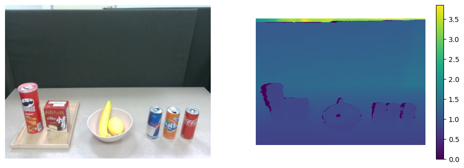
Fig. 1: RGBD image
Detect tag
위 과정을 통해 기본적으로 RGBD 이미지를 받아올 수 있게 되었다. 그 다음 과정으로는 tag detection이다. Pose estimation을 위해서는 tag부터 명확하게 검출할 수 있어야하며, 당연히 tag가 검출된 이후에 pose를 추정할 수 있다. 아래는 tag detection 코드이다. (검출된 tag 기준의 bounding cude 함수도 구현하였다.)
import apriltag

def _draw_cube(overlay, camera_params, tag_size, pose, z_sign=1):
    """
        Draw the cube of the tag.
    """
    # object points
    opoints = np.array([
        -1, -1, 0,          # Lower points
         1, -1, 0,
         1,  1, 0,
        -1,  1, 0,
        -1, -1, -2*z_sign,  # Upper points
         1, -1, -2*z_sign,
         1,  1, -2*z_sign,
        -1,  1, -2*z_sign,
    ]).reshape(-1, 1, 3) * 0.5*tag_size

    # image points
    edges = np.array([
        0, 1,
        1, 2,
        2, 3,
        3, 0,
        0, 4,
        1, 5,
        2, 6,
        3, 7,
        4, 5,
        5, 6,
        6, 7,
        7, 4
    ]).reshape(-1, 2)

    fx, fy, cx, cy = camera_params
    K = np.array([fx, 0, cx, 0, fy, cy, 0, 0, 1]).reshape(3, 3)
    rvec, _ = cv2.Rodrigues(pose[:3,:3])
    tvec = pose[:3, 3]

    dcoeffs = np.zeros(5)
    ipoints, _ = cv2.projectPoints(opoints, rvec, tvec, K, dcoeffs)
    ipoints = np.round(ipoints).astype(int)
    ipoints = [tuple(pt) for pt in ipoints.reshape(-1, 2)]

    for i, j in edges:
        cv2.line(overlay, ipoints[i], ipoints[j], (0, 255, 0), 1, 16)

def meters2xyz(depth_img,camera_info):
    """
        Scaled depth image to pointcloud
    """
    fx = camera_info.fx
    cx = camera_info.ppx
    fy = camera_info.fx
    cy = camera_info.ppy

    height = camera_info.height
    width = camera_info.width

    indices = np.indices((height, width),dtype=np.float32).transpose(1,2,0)

    z_e = depth_img
    x_e = (indices[..., 1] - cx) * z_e / fx
    y_e = (indices[..., 0] - cy) * z_e / fy

    # scale to meter unit.
    xyz_img = np.stack([-y_e*0.001, -x_e*0.001, z_e*0.001], axis=-1) # Shape: [H x W x 3]
    return xyz_img # [H x W x 3]

# apriltag setting.
detector = apriltag.Detector()
tag_size = 0.035 # Tag size: Diameter
img_xyz_clipped_filled = meters2xyz(depth_clipped_filled, camera_info=intrinsic_matrix_depth)

img_copy = copy.deepcopy(color_image)
img_bgr = cv2.cvtColor(img_copy, cv2.COLOR_RGB2BGR)
img_gray = cv2.cvtColor(img_bgr, cv2.COLOR_BGR2GRAY)
img_xyz = meters2xyz(depth_clipped_filled, camera_info=intrinsic_matrix_depth)

results, dimg = detector.detect(img_gray, return_image=True)
if len(img_copy.shape) == 3:
    overlay = img_copy // 2 + dimg[:, :, None] // 2
else:
    overlay = img_copy // 2 + dimg // 2

for r in results:
    pose, e0, e1 = detector.detection_pose(detection=r, camera_params=cam_params_rgb, tag_size=tag_size)    # should check tag_size
    center_uv = (int(r.center[0]), int(r.center[1]))
    _draw_cube(overlay,
                cam_params_rgb,
                tag_size,
                pose)
cv2.namedWindow('Tag Detection Example', cv2.WINDOW_AUTOSIZE)
cv2.imshow('Tag Detection Example', overlay)

key = cv2.waitKey(1)
if key & 0xFF == ord('q') or key == 27:
    cv2.destroyAllWindows()
    break
위 코드의 results, dimg = detector.detect(img_gray, return_image=True) 를 통해 입력 이미지 img_gray에 있는 tag를 검출하게 된다. 우선 gray scale의 이미지를 사용하는 이유는 다음과 같다.
- color 채널이 제거되며, 패턴을 더욱 뚜렷하게 표현할 수 있다.
- 일반적으로 패턴을 검출할 때에는 인접 픽셀 값의 차이를 사용하는데, gray 채널은 픽셀 당 하나의 값을 가지므로 연산이 간단하고 빨라진다.
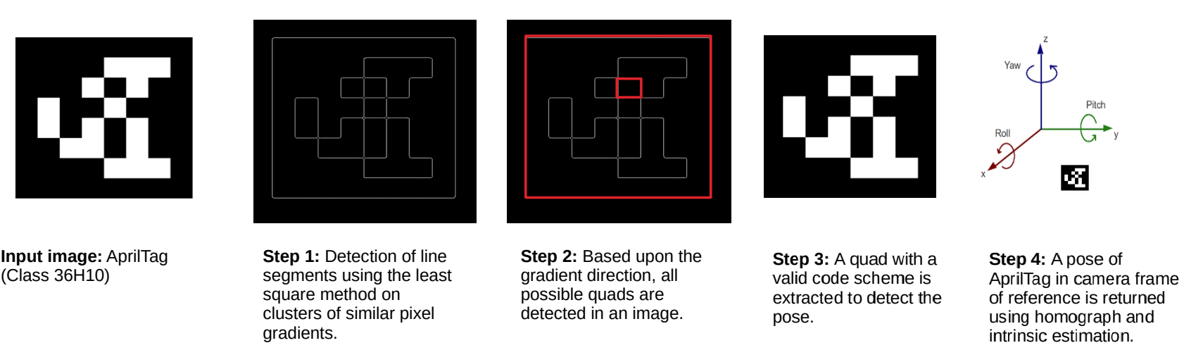
Fig. 2: Overall algorithm of AprilTag
검출된 tag에 대한 정보는 dictionary 형태로 얻어지며, 각 내용은 아래와 같다.
Detection(tag_family=b'tag36h11',
          tag_id=0,
          hamming=0,
          goodness=0.0,
          decision_margin=105.59999084472656,
          homography=array([[ -0.81,   0.36, -11.45],
                            [  0.  ,  -0.32,  -8.8 ],
                            [  0.  ,   0.  ,  -0.02]]),
          center=array([582.71, 448.03]),
          corners=array([[543.41, 418.91],
                         [623.08, 418.91],
                         [624.49, 478.99],
                         [539.82, 478.99]]))
각각에 해당하는 용어 설명은 아래와 같다.
<!DOCTYPE html>
| Attribute | Explanation |
|---|---|
| tag_family | The family of the tag. |
| tag_id | The decoded ID of the tag. |
| hamming | How many error bits were corrected? Note: accepting large numbers of corrected errors leads to greatly increased false positive rates. NOTE: As of this implementation, the detector cannot detect tags with a Hamming distance greater than 3. |
| decision_margin | A measure of the quality of the binary decoding process: the average difference between the intensity of a data bit versus the decision threshold. Higher numbers roughly indicate better decodes. This is a reasonable measure of detection accuracy only for very small tags -- not effective for larger tags (where we could have sampled anywhere within a bit cell and still gotten a good detection.) |
| homography | The 3x3 homography matrix describing the projection from an "ideal" tag (with corners at (-1,1), (1,1), (1,-1), and (-1,-1)) to pixels in the image. |
| center | The center of the detection in image pixel coordinates. |
| corners | The corners of the tag in image pixel coordinates. These always wrap counter-clockwise around the tag. |
아래는 tag detection 결과이며, 직관적인 이해를 위해 tag를 둘러싸는 cube도 그려보았다.
Pose Estimation
마지막으로, 검출된 tag 정보를 기반으로 tag의 pose도 손쉽게 알아낼 수 있다. 해당 함수는 detector.detection_pose(detection=r, camera_params=cam_params_rgb, tag_size=tag_size) 이며, 이에 해당하는 4x4 pose matrix와 오차값 \(\mathrm{e_{1}},~\mathrm{e_{2}}\) 를 내어준다.
apriltag 모듈로 들어가, 해당 함수를 조금 더 자세히 분석해보면 어떻게 tag pose를 얻어오는지 이해할 수 있다. 해당 함수의 코드만 가져왔으며, class Detector의 멤버함수이다.
def detection_pose(self, detection, camera_params, tag_size=1, z_sign=1):

    fx, fy, cx, cy = [ ctypes.c_double(c) for c in camera_params ]

    H = self.libc.matd_create(3, 3)
    arr = _matd_get_array(H)
    arr[:] = detection.homography
    corners = detection.corners.flatten().astype(numpy.float64)

    dptr = ctypes.POINTER(ctypes.c_double)

    corners = corners.ctypes.data_as(dptr)

    init_error = ctypes.c_double(0)
    final_error = ctypes.c_double(0)

    Mptr = self.libc.pose_from_homography(H, fx, fy, cx, cy,
                                          ctypes.c_double(tag_size),
                                          ctypes.c_double(z_sign),
                                          corners,
                                          dptr(init_error),
                                          dptr(final_error))

    M = _matd_get_array(Mptr).copy()
    self.libc.matd_destroy(H)
    self.libc.matd_destroy(Mptr)

    return M, init_error.value, final_error.value
코드를 보면 알 수 있듯이, camera의 intrinsic parameter와 검출된 tag의 homography matrix 정보 만으로 pose를 추정해낼 수 있다. homography matrix를 구하는 과정과 정의는 다음과 같다.
How to get Homography matrix?
- 논문에서 밝히길,
Homography matrix는Direct Linear Transform (DLT)방법론으로 구한다고 한다.DLT란 Four point correspondences \(x_{i}\), \(x_{i}'\) 가 주어질 때에. \(H x_{i} = x_{i}'\) 이면, \(x_{i}' \times H x_{i} = 0\) 이 성립한다는 것이다.Definition of Homography matrix Briefly, the planar homography relates the transformation between two planes (up to a scale factor):
\[\begin{equation*} s \begin{bmatrix} x' \\ y' \\ 1 \end{bmatrix} = \mathbf{H} \begin{bmatrix} x \\ y \\ 1 \end{bmatrix} = \begin{bmatrix} h_{11} & h_{12} & h_{13} \\ h_{21} & h_{22} & h_{23} \\ h_{31} & h_{32} & h_{33} \end{bmatrix} \begin{bmatrix} x \\ y \\ 1 \end{bmatrix} \end{equation*}\]The homography matrix is a 3x3 matrix but with 8 DoF (degrees of freedom) as it is estimated up to a scale. It is generally normalized (see also 1) with \(h_{33}=1\) or \(h_{11}^2 + h_{12}^2 + h_{13}^2 + h_{21}^2 + h_{22}^2 + h_{23}^2 + h_{31}^2 + h_{32}^2 + h_{33}^2 = 1\)
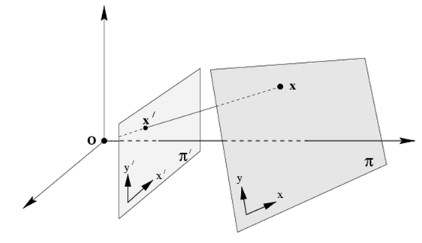
Fig. 3: a planar surface and the image plane
즉, planar surface와 image plane을 matching 해주는 matrix라고 생각하면 된다. 내가 사용한 RealSense D435i 카메라는 양안 렌즈이며, rgb_camera와 depth_camera의 intrinsic parameter가 개별적으로 설정되어 있다. 이는 pyrealsense2 module로 손쉽게 구할 수 있으며, 이에 해당하는 코드는 아래와 같다.
import pyrealsense2 as rs
import matplotlib.pyplot as plt
import numpy as np
import cv2
import copy
from utils.util import r2rpy, rpy2r, r2t, t2r, pr2t

pipeline = rs.pipeline()
config = rs.config()
config.enable_stream(rs.stream.depth, 640, 480, rs.format.z16, 30) # Order: [H x W]
config.enable_stream(rs.stream.color, 640, 480, rs.format.bgr8, 30) # Order: [H x W]

profile = pipeline.start(config)
stream_depth = profile.get_stream(rs.stream.depth)

### Camera Parameters
intrinsic_matrix_depth = stream_depth.as_video_stream_profile().get_intrinsics()
intrinsic_matrix_rgb = profile.get_stream(rs.stream.color).as_video_stream_profile().get_intrinsics()

cam_params_depth = [intrinsic_matrix_depth.fx, intrinsic_matrix_depth.fy, intrinsic_matrix_depth.ppx, intrinsic_matrix_depth.ppy]
cam_params_rgb = [intrinsic_matrix_rgb.fx, intrinsic_matrix_rgb.fy, intrinsic_matrix_rgb.ppx, intrinsic_matrix_rgb.ppy]
cam_matrix_depth = np.array([[intrinsic_matrix_depth.fx, 0, intrinsic_matrix_depth.ppx],
                        [0, intrinsic_matrix_depth.fy, intrinsic_matrix_depth.ppy],
                        [0, 0, 1]])
cam_matrix_rgb = np.array([[intrinsic_matrix_rgb.fx, 0, intrinsic_matrix_rgb.ppx],
                        [0, intrinsic_matrix_rgb.fy, intrinsic_matrix_rgb.ppy],
                        [0, 0, 1]])
pyrealsense를 사용하지 않고, ros topic로도 손쉽게 정보를 얻어올 수 있다. 그러기 위해서는 ROS로 D435i와 연결해주어야 하며, 해당하는 터미널 라인은 아래와 같다.
ros2 run realsense2_camera realsense2_camera_node
잘 연결 되었다면, 아래의 터미널 라인을 통해 각각에 해당하는 camera parameter를 얻어올 수 있다. (자세한 정보는 공식 레포에서 확인할 수 있다.)
ros2 topic echo /color/camera_info
ros2 topic echo /depth/camera_info
각각의 토픽에서 어떠한 내용을 갖고있는지는 ROS realsense_camera wiki에서 자세한 정보를 알 수 있다.
/color/camera_info & /depth/camera_info | Explanation |
|---|---|
std_msgs/Header header | Time of image acquisition, camera coordinate frame ID |
uint32 height & uint32 width | The image dimensions with which the camera was calibrated. Normally this will be the full camera resolution in pixels. |
string distortion_model | The distortion model used. Supported models are listed in sensor_msgs/distortion_models.h. For most cameras, “plumb_bob” - a simple model of radial and tangential distortion - is sufficient. |
float64[] D | The distortion parameters, size depending on the distortion model. For “plumb_bob”, the 5 parameters are: (k1, k2, t1, t2, k3). |
float64[9] K | # Intrinsic camera matrix for the raw (distorted) images. Projects 3D points in the camera coordinate frame to 2D pixel coordinates using the focal lengths (fx, fy) and principal point (cx, cy). |
float64[9] R | Rectification matrix (stereo cameras only). A rotation matrix aligning the camera coordinate system to the ideal stereo image plane so that epipolar lines in both stereo images are parallel. |
float64[12] P | Projection/camera matrix. By convention, this matrix specifies the intrinsic (camera) matrix of the processed (rectified) image. That is, the left 3x3 portion is the normal camera intrinsic matrix for the rectified image. It projects 3D points in the camera coordinate frame to 2D pixel coordinates using the focal lengths (fx’, fy’) and principal point (cx’, cy’) - these may differ from the values in K. |
uint32 binning_x & uint32 binning_y | Binning refers here to any camera setting which combines rectangular neighborhoods of pixels into larger “super-pixels.” It reduces the resolution of the output image to (width / binning_x) x (height / binning_y). The default values binning_x = binning_y = 0 is considered the same as binning_x = binning_y = 1 (no subsampling). |
sensor_msgs/RegionOfInterest roi | Region of interest (subwindow of full camera resolution), given in full resolution (unbinned) image coordinates. A particular ROI always denotes the same window of pixels on the camera sensor, regardless of binning settings. The default setting of roi (all values 0) is considered the same as full resolution (roi.width = width, roi.height = height). |
당연하게도, 여기서 사용되는 intrinsic parameter는 rgb_camera의 정보를 사용해야만 한다. (입력으로 넣어주었던 이미지가 rgb_camera에서 얻어온 것이므로.)
pose_from_homography 함수에 대한 c++ code는 OpenCV 공식 페이지에서 확인할 수 있다.
Homography matrix로 pose estimation을 하는 과정은 Multiple View Geometry in Computer Vision Second Edition의 Sec. 9.6.2에서 확인할 수 있다.
위에서 구한 Homography matrix를 통해 상대적인 pose [R|t]를 구하기 위하여 Singular Value Decomposition(SVD)을 활용합니다. SVD는 행렬을 대학화하는 방법 중 하나이다.
-
Homogeneous Coordinates (동차 좌표계):
- 먼저, 카메라와 3D point 간의 관계를 표현하기 위해
동차 좌표계를 사용한다. 3D point는 \((X, Y, Z, 1)^T\)와 같이 표현되며, 2D image point는 \((x, y, 1)^T\)로 표현된다.
- 먼저, 카메라와 3D point 간의 관계를 표현하기 위해
-
Homography Equation:
-
Homography 행렬 H는 다음과 같은 관계를 나타낸다:
\[\begin{equation*} \begin{bmatrix} s \cdot x' \\ s \cdot y' \\ s \end{bmatrix} = s \begin{bmatrix} x' \\ y' \\ 1 \end{bmatrix} = \mathbf{H} \begin{bmatrix} X \\ Y \\ Z \\ 1 \end{bmatrix} \end{equation*}\] -
여기서 \((x', y')\)는 image plane 상의 2D point이고 \((X, Y, Z)\)는 3D 공간 상의 3D point이다. \(s\)는 스케일 요소로, 일반적으로 1로 설정된다.
-
-
Homography Decomposition:
-
Homography matrix\(\mathrm{H}\)의 분해는 rotational matrix \(\mathrm{R}\)과 translational vector \(\text{tvec}\)으로 이루어진다. - Decomposition 과정은 아래와 같이 수행된다. \(\begin{equation*} \mathbf{H} = \mathbf{K} \left[ \begin{array}{ccc|c} r_{11} & r_{12} & r_{13} & t_x \\ r_{21} & r_{22} & r_{23} & t_y \\ r_{31} & r_{32} & r_{33} & t_z \\ \end{array} \right] \end{equation*}\) 여기서 \(\mathbf{K}\)는 camera intrinsic matrix이고, \(r_{ij}\)는 회전 행렬 \(\mathrm{R}\)의 각 요소이다.
-
-
Polar Decomposition:
- 회전 행렬 \(\mathrm{R}\)에 대해
polar decomposition을 사용하여orthonormal matrix로 분해한다.polar decomposition는 \(\mathrm{R}\)을SVD과정으로 \(\mathrm{R} = \mathrm{U} \cdot \mathrm{V^T}\)로 분해한다.- 특이값 분해에서 얻은 \(\mathrm{U}\)와 \(\mathrm{V}\)를 사용하여 보정된 \(\mathrm{R}\)을 계산하며, 보정된 회전 행렬 \(\mathrm{R'}\)은 다음과 같이 수행된다. \(\begin{equation*} \mathrm{R'} = \frac{1}{\text{det}(\mathrm{V^T})} \cdot \mathrm{U} \end{equation*}\)
- 회전 행렬 \(\mathrm{R}\)에 대해
-
Get
rvec:- 보정된 회전 행렬 \(\mathrm{R'}\)을 사용하여
Rodrigues변환을 사용하여 회전 벡터rvec으로 변환한다.
- 보정된 회전 행렬 \(\mathrm{R'}\)을 사용하여
이렇게 긴 과정을 거쳐, AprilTag의 pose가 검출된다. 검출된 tag의 pose는 camera coordinate 기준이며, 이는 각자가 설정한 base(=world) coordinate로 transformation 과정을 마지막으로 수행해주면, tag의 pose를 얻어낼 수 있게 된다.
검출된 Tag의 center point를 base(=world) coordinate 기준으로 계산된 \((x,y,z)_{\text{world}}\) 를 실시간으로 우측 상단에 배치하였다. 나는 MuJoCo의 coordination을 world coordinate로 삼았으며, 이는 아래와 같다.
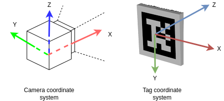
Fig. 4: Coordination
- Coordination of MuJoCo Engine
- \(\mathrm{X}\): Out of the camera
- \(\mathrm{Y}\): Left
- \(\mathrm{Z}\) : Up
- Coodination of AprilTag
- \(\mathrm{X}\): Right
- \(\mathrm{Y}\): Down
- \(\mathrm{Z}\) : Into the Tag
- In the official repository,
The coordinate system has the origin at the camera center. The z-axis points from the camera center out the camera lens. The x-axis is to the right in the image taken by the camera, and y is down. The tag’s coordinate frame is centered at the center of the tag, with x-axis to the right, y-axis down, and z-axis into the tag.
- In the official repository,
잘 안 보이겠지만, 줄자로 길이를 가늠해보았을 때 실제 scale에 맞게 Translational 정보를 잘 추정하는 것을 알 수 있다.
Fig. 5: Table configuration.
Enjoy Reading This Article?
Here are some more articles you might like to read next: