[study] Mixture Density Network
0. Simple Networks
일반적으로 네트워크를 구성한다는 것은 입력과 출력에 대해 설계하는 것이다. 이를 조건부 확률로 나타내면 다음과 같다.
\[p(y|x,z)\]- \(x\): Input of the network
- \(z\): Model parameter
- \(y\): Output of the network (=label)
예를 들어, 만일 classification 문제를 수행하고 있다면 \(y\)는 분류해야 할 label을 의미하는 것이다. 각 label은 discrete하게 존재하므로 (e.g., dog or cat) 출력 값에 Softmax 연산을 수행해주어 어떠한 class에 해당할 확률을 뱉어주게 된다.
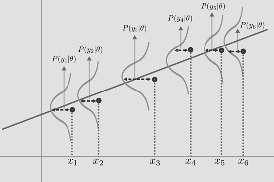
Fig. 1: Simple image about Linear Regression.
Regression 문제를 수행하고 있다면 출력 값 \(y\)는 continuous 한 값을 갖게 될 것이다. 어떠한 입력 \(x\)에 대응하는 출력 \(y\)의 값이 있을 것이며, 이에 대해 Mean Squared Error (MSE)로 선형회귀를 수행한다면 주어진 입력 \(x\)에 대해 가장 잘 표현하는 직선을 얻게 될 것이다.
실제 직선을 \(f(x)\)라고 칭하고, 예측한 직선을 \(\hat{f}(x)\) 라고 한다면 두 직선 간의 차이는 존재하게 된다. \(f(x) = \hat{f}(x) + \epsilon\) 완벽하게 일치하는 직선은 존재할 수 없으며, 작은 오차 \(\epsilon\)을 가지게 되며, 이러한 오차는 (보통) Gaussian distribution을 따른다고 가정한다. 이를 확률 분포로 표현하면 아래와 같으며, \(w\)는 각각의 weight를 의미한다.
\[\left( y \mid x \right) \sim N(w^Tx, \sigma^2)\]0.1. Example: Simple Sinusoidal Function
\[\begin{equation} y_{\text{true}}(x) = 7\sin{(0.75x)} + 0.5x + \epsilon \end{equation}\]위 함수를 기준으로 Regression 문제를 수행해보자.
import matplotlib.pyplot as plt
import numpy as np
import torch
import torch.nn as nn
from torch.autograd import Variable

def sample_data(n_samples):
    epsilon = np.random.normal(size=(n_samples))
    x_data = np.random.uniform(-10.5, 10.5, n_samples)
    y_data = 7*np.sin(0.75*x_data) + 0.5*x_data + epsilon
    return x_data, y_data

n_samples = 1000
x_data, y_data = sample_data(n_samples)

plt.figure(figsize=(8, 8))
plt.scatter(x_data, y_data, alpha=0.2)
plt.show()
위 코드를 통해 위 함수에 근사하는 데이터를 추출할 수 있었다.
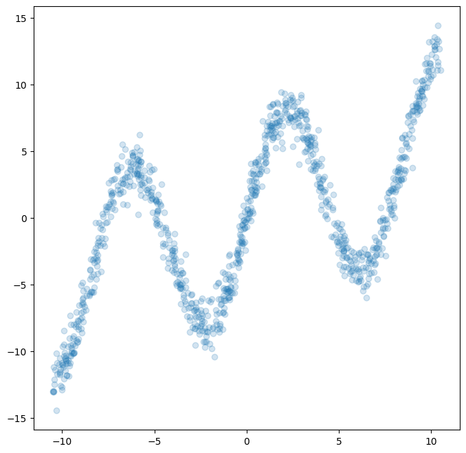
Fig. 2: Sampled from arbitrary function.
그럼 이제 이 함수를 근사할 수 있는 간단한 네트워크를 구성해볼 수 있다.
n_input = 1
n_hidden = 20
n_output = 1

network = nn.Sequential(nn.Linear(n_input, n_hidden),
                        nn.Tanh(),
                        nn.Linear(n_hidden, n_output))
optimizer = torch.optim.Adam(network.parameters())
loss_fn = nn.MSELoss()

x_tensor = torch.from_numpy(np.float32(x_data).reshape(n_samples, n_input))
y_tensor = torch.from_numpy(np.float32(y_data).reshape(n_samples, n_input))
x_variable = Variable(x_tensor)
y_variable = Variable(y_tensor, requires_grad=False)

def train():
    for epoch in range(3000):
        y_pred = network(x_variable)
        loss = loss_fn(y_pred, y_variable)
        optimizer.zero_grad()
        loss.backward()
        optimizer.step()

        if epoch % 300 == 0:
            print(epoch, loss.data[0])
간단한 MLP layer를 만들어, MSE Loss를 최소화하도록 학습시킨다. 이때 주의할 점은 numpy array를 pytorch가 사용할 수 있는 tensor로 바꿔줘야한다. 또한 numpy의 기본 형태인 np.float64를 pytorch의 기본형인 np.float32로 바꿔줘야 에러가 발생하지 않는다.
train()

x_test_data = np.linspace(-10, 10, n_samples)
x_test_tensor = torch.from_numpy(np.float32(x_test_data).reshape(n_samples, n_input))
x_test_variable = Variable(x_test_tensor)
y_test_variable = network(x_test_variable)
y_test_data = y_test_variable.data.numpy()

plt.figure(figsize=(8, 8))
plt.scatter(x_data, y_data, alpha=0.2)
plt.scatter(x_test_data, y_test_data, alpha=0.2)
plt.show()
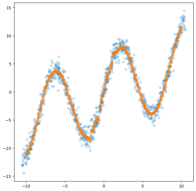
Fig. 3: Fitted with simple network.
이는 간단하게 학습된 네트워크에 test input \(x\)를 샘플하여 정말 잘 학습 되었는지 확인하는 코드이다. 위 그림을 보면 알 수 있듯이, 손쉽게 해당 function에 fitting 된 것을 알 수 있다. 이론 상으로는 은닉층 하나 만으로도 MLP는 임의의 함수를 근사할 수 있다는 점을 알 수 있다. 즉, 하나 이상의 input \(x\)와 그에 대응하는 오직 하나의 출력 \(y\)을 갖는 함수에 대해서는 쉽게 표현할 수 있다는 것을 의미한다.
다르게 생각해보면, 여러 개의 출력을 갖는 경우에는 어떻게 될지 생각해볼 수 있다. 즉 앞선 경우는 mode가 1인 경우에 regression을 수행한 것이며, 여러 개의 mode로 표현되는 정규분포에 대해 regression을 수행할 때에도 정말 잘 표현할 수 있는지는 고민해볼 필요가 있다.
0.2. Example: Reverse of the Eqn. 1
plt.figure(figsize=(8, 8))
plt.scatter(y_data, x_data, alpha=0.2)
plt.show()
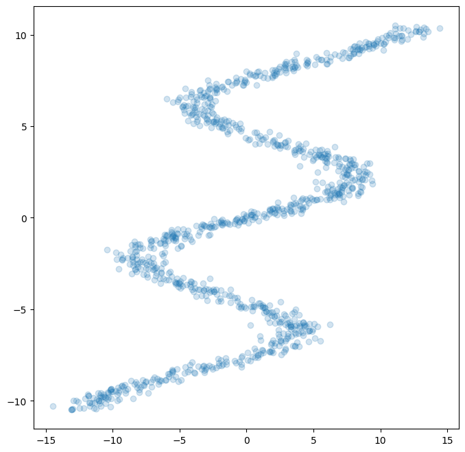
Fig. 4: Reverse of the function.
간단하게 \(x\)와 \(y\)를 서로 바꾸어주면 된다. 이렇게 되면 하나의 입력 \(x\)는 여러 개의 출력 \(y\)를 표현하게 된다. 이러한 상황에서 기존의 네트워크를 사용하여 다시 학습해보자.
x_variable.data = y_tensor
y_variable.data = x_tensor

train()

x_test_data = np.linspace(-15, 15, n_samples)
x_test_tensor = torch.from_numpy(np.float32(x_test_data).reshape(n_samples, n_input))
x_test_variable.data = x_test_tensor

y_test_variable = network(x_test_variable)

# move from torch back to numpy
y_test_data = y_test_variable.data.numpy()

# plot the original data and the test data
plt.figure(figsize=(8, 8))
plt.scatter(y_data, x_data, alpha=0.2)
plt.scatter(x_test_data, y_test_data, alpha=0.2)
plt.show()
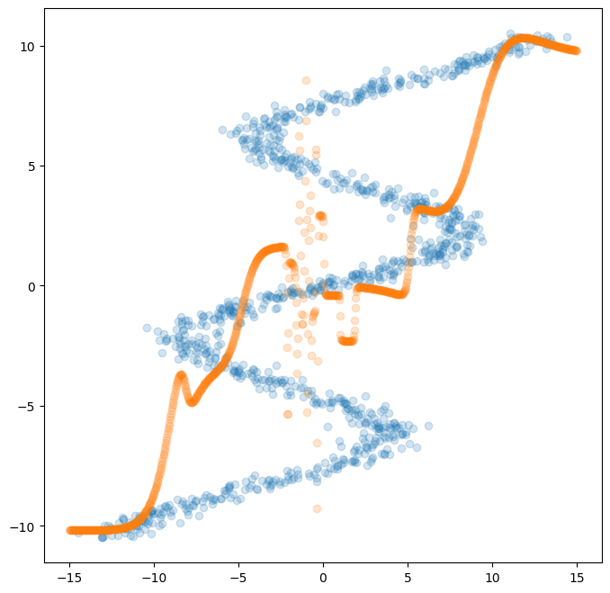
Fig. 5: Result with simple network.
이렇게 여러 mode의 distribution에 대해서는 일반적인(간단한) 네트워크로는 표현하기 어렵다는 것을 알 수 있다. 이는 기본적으로 MSE Loss를 최소화하도록 학습시키고 각 입력에 대해 하나의 출력만 가능했기 때문이다. 이러한 문제를 해결하기 위해서 제안된 것이 Mixture Density Network (MDN) 이다.
1. Mixture Density Network (MDN)
1.1 Definition
| MDN은 paper에서 자세한 내용을 확인할 수 있다. 정리하면, 하나의 입력 \(x\)에 대해 다른 분포를 가지는 \(y\)에서 $$p(y | x)$$를 추정하는 것이다. |
이를 수식으로 표현하면 위와 같으며, \(n\)개의 정규분포를 가정하고 각 분포에서 \(y\)가 나올 확률을 이 분포에 속할 확률과 곱하여 결과를 예측하는 것이다. 이렇게 \(p(y \mid x)\)를 얻어, 여기서 sample 하여 함수를 추정하면 끝이다.
그렇게 Network에서 결정(추정)해주어야 할 값은 총 3가지 이다. (각 분포마다 3개씩.)
- \(p(c=i \mid x)\): 입력 \(x\)가 category \(i\)에 속할 확률.
- 확률분포의 정의에 의해 Normalize를 반드시 해주어야 한다. (총 합이 1이 되게끔 softmax를 수행함.)
- \(\mu^{i},~\sigma^{i}\): category \(i\)에 속할 때 \(y\)가 따르는 정규분포
- \[\sigma^{i} > 0\]
그리고 이젠 출력이 단일한 값을 뱉어주지 못하므로 loss 또한 MSE Loss가 아닌 다른 loss를 사용해야 한다. Cross-Entropy Loss를 사용하며, 수식은 아래와 같다.
\[\begin{equation} \mathcal{L}_{\text{C.E.}} = -\log{ \sum_{i=1}^m p(c = i \mid x)N(y; \mu^i, \sigma^i)} \end{equation}\]그렇다면 위 loss function을 가지며, Network의 출력은 \(\pi,~\mu,~\sigma\)를 하는 MDN class를 만든다.
class MDN(nn.Module):
    def __init__(self, n_hidden, n_gaussians):
        super(MDN, self).__init__()
        self.z_h = nn.Sequential(
            nn.Linear(1, n_hidden),
            nn.Tanh()
        )
        self.z_pi = nn.Linear(n_hidden, n_gaussians)
        self.z_mu = nn.Linear(n_hidden, n_gaussians)
        self.z_sigma = nn.Linear(n_hidden, n_gaussians)

    def forward(self, x):
        z_h = self.z_h(x)
        pi = nn.functional.softmax(self.z_pi(z_h), -1)
        sigma = torch.exp(self.z_sigma(z_h))
        mu = self.z_mu(z_h)
        return pi, sigma, mu
-
z_pi는 확률분포 이기에 softmax를 수행해준 것이다. -
z_sigma는 항상 양수이어야 하므로 \(\exp\)를 취해주었다.
\(\mu^{i},~\sigma^{i}\)에서 정의되는 정규분포의 수식은 아래와 같다.
\[\begin{equation*} \mathcal{N}(\mu, \sigma)(x) = \frac{1}{\sigma \sqrt{2\pi}} \exp (-\frac{(x-\mu)^2}{2\sigma^2}) \end{equation*}\]이를 고려한 loss function을 코드로 구현하면 아래와 같다.
def gaussian_distribution(y, mu, sigma):
    result = (y.expand_as(mu) - mu) * torch.reciprocal(sigma)
    result = -0.5 * (result * result)
    return (torch.exp(result) * torch.reciprocal(sigma)) * 1.0 / np.sqrt(2.0*np.pi)

def mdn_loss_fn(pi, sigma, mu, y):
    result = gaussian_distribution(y, mu, sigma) * pi
    result = torch.sum(result, dim=1)
    result = -torch.log(result)
    return torch.mean(result)
각 분포로부터 \(y\)가 나올 확률 \(\mathcal{N}(\mu,\sigma)(x)\)와 그 분포에 대응할 확률 \(\pi\)을 곱하고, 이 모두를 다 더한 다음, 로그와 평균을 취해주면 된다.
network = MDN(n_hidden=20, n_gaussians=5)
optimizer = torch.optim.Adam(network.parameters())

mdn_x_data = y_data
mdn_y_data = x_data

mdn_x_tensor = y_tensor
mdn_y_tensor = x_tensor

x_variable = Variable(mdn_x_tensor)
y_variable = Variable(mdn_y_tensor, requires_grad=False)

def train_mdn():
    for epoch in range(10000):
        pi_variable, sigma_variable, mu_variable = network(x_variable)
        loss = mdn_loss_fn(pi_variable, sigma_variable, mu_variable, y_variable)
        optimizer.zero_grad()
        loss.backward()
        optimizer.step()

        if epoch % 500 == 0:
            print(epoch, loss.data[0])

train_mdn()

pi_variable, sigma_variable, mu_variable = network(x_test_variable)

pi_data = pi_variable.data.numpy()
sigma_data = sigma_variable.data.numpy()
mu_data = mu_variable.data.numpy()

fig, (ax1, ax2, ax3) = plt.subplots(3, 1, sharex=True, figsize=(8,8))
ax1.plot(x_test_data, pi_data)
ax1.set_title('$$p(c = i | x)$$')
ax2.plot(x_test_data, sigma_data)
ax2.set_title('$$\sigma$$')
ax3.plot(x_test_data, mu_data)
ax3.set_title('$$\mu$$')
plt.xlim([-15,15])
plt.show()
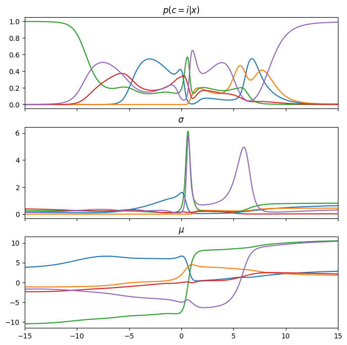
Fig. 6: Result with MDN network.
입력 \(x\)의 변화에 따른 각 분포의 양상을 확인할 수 있다. 하나의 \(x\)에 여러 개의 \(y\)가 가능하며, 이 각각의 점이 선택될 확률은 \(\mathbf{p(c=i \mid x)}\)로 표현되는 것이다.
학습시킨 네트워크에서 특정 정규분포의 결과를 얻고 싶다면 Gumbel softmax sampling을 사용하면 되며, 이론적인 내용은 이후에 작성하겠습니다.
이제 우리는 각 입력 \(x\)에 대해서 어떤 정규분포를 선택해야되는지를 알았으니 각각의 평균과 분산을 이용해 이를 sampling만 하면 됩니다. random noise는 표준정규분포를 따르므로 이에 \(\sigma\)를 곱하고 \(\mu\)를 더해주기만하면 원래의 정규분포를 얻을 수 있다. 이렇게 해서 최종 결과물을 시각화하면 아래와 같다.
def gumbel_sample(x, axis=1):
    z = np.random.gumbel(loc=0, scale=1, size=x.shape)
    return (np.log(x) + z).argmax(axis=axis)

k = gumbel_sample(pi_data)

indices = (np.arange(n_samples), k)
random_noise = np.random.randn(n_samples)
sampled = random_noise * sigma_data[indices] + mu_data[indices]

plt.figure(figsize=(8, 8))
plt.scatter(mdn_x_data, mdn_y_data, alpha=0.2)
plt.scatter(x_test_data, sampled, alpha=0.2, color='red')
plt.show()
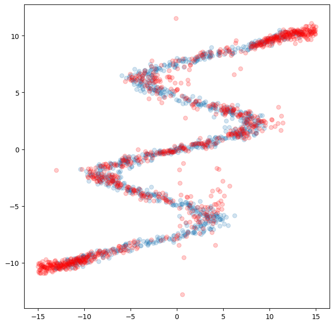
Fig. 7: Fitted with MDN network.
요약
기존의 간단한 network는 하나의 입력 \(\mathbf{x}\)에 대해 여러 개의 출력 \(\mathbf{y}\)가 가능한 경우에 효과적으로 표현할 수 없었다. Mixture Density Network (MDN)은 여러 개의 정규분포 \(\mathbf{\mathcal{N}^{i}}\) (혹은 다른 분포)의 평균 \(\mathbf{\mu}^{i}\)와 분산 \(\mathbf{\sigma}^{i}\)를 예측하고, 각 정규분포에 속할 확률 \(\mathbf{\pi^{i}=p(c=i \mid x)}\)을 통해 이를 효과적으로 근사할 수 있게 한 것이다. 즉, 여러 개의 출력이 있는 경우에도 분포를 추정할 수 있다는 의미이다.
References:
Enjoy Reading This Article?
Here are some more articles you might like to read next: