[study] Vector Quantization

1. Vector quantization (VQ)

1.1. In what applications is VQ used?

Vector quantization is used in many applications such as image and voice compression, voice recognition (in general statistical pattern recognition), and surprisingly enough in volume rendering.

1.2. Definition: What is VQ?

A vector quantizer maps k-dimensional vectors in the vector space \(\mathbb{R}^{k}\) into a finite set of vectors \(Y = \{y_{i}: i = 1, 2, \cdots, N\}\). Each vector \(y_{i}\) is called a code vector or a codeword. and the set of all the codewords is called a codebook. Associated with each codeword, \(y_{i}\), is a nearest neighbor region called Voronoi region, and it is defined by:

Suppose you have recorded sounds at different locations and want to categorize them into similar groups. In other words, you have a stochastic vector \(x\) which you want to characterize with a simple description. For example, categories could correspond to \(\textbf{office, street, hallway}\) and \(\textbf{cafeteria}\).

A classic way for this task is to choose template vectors \(\mathbf{c_{k}}\), which represents a typical sound in each environment \(\mathbf{k}\). To categorize the sounds, you then find that template vector which is closest to your recording \(\mathbf{x}\). In mathematical notation, you search for a \(\mathbf{ k^{^*} }\) by

\[\mathbf{k^*} = \arg\min_{\mathbf{k}} \|x-c_{\mathbf{k} }\|^2.\]

The above expression thus calculates the squared error between \(x\) and each of the vectors \(c_{\mathbf{k}}\) and chooses the index \(\mathbf{k}\) of the vector with the smallest error. The vectors \(c_{\mathbf{k}}\) then represent a codebook and the vector \(x\) is quantized to \(c_{\mathbf{k}^*}\). This is the basic idea behind vector quantization, which is also known as \(\mathbf{k}\)-means.

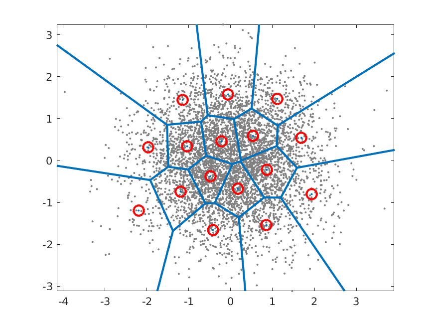
Fig. 1: Example of a codebook for a 2D Gaussian with 16 code vectors.

A illustration of a simple vector codebook is shown on the above. The input data is a Gaussian distribution shown with grey dots and the codebook vectors \(c_{\mathbf{k}}\) with red circles. For each input vector we thus search for the nearest codebook vector and the borders of the regions where input vectors are assigned to a particular codebook vector are illustrated with blue lines. These regions are known as Voronoi regions and the blue lines are the decision-boundaries between codebook vectors.

1.3. Metric for codebook quality

Suppose then that you have a large collection of vectors \(x_{h}\), and you want to find out how well this codebook represents the input data. The expectation of the squared error is approximately the mean over your data, such that

\[E_h\left[ \min_\mathbf{k} \|x_h-c_\mathbf{k}\|^2 \right] \approx \frac 1N \sum_{h=1}^N \min_\mathbf{k} \|x_h-c_\mathbf{k}\|^2,\]

where \(E[\cdot]\) is the expectation operator and \(N\) is the number of input vectors \(x_{h}\). Above, we thus find the codebook vector which is closest to \(x_{h}\), find its squared error and take the expectation over all possible inputs. This is approximately equal to the mean of those squared errors over a set of input vectors. To find the best set of codebook vectors \(c_{k}\), we then need to minimize the mean squared error as

\[\{c_\mathbf{k}^*\} := \arg\min_{\{c_\mathbf{k}\}}\, E_h\left[ \min_\mathbf{k} \|x_h-c_\mathbf{k}\|^2 \right]\]

or more specifically, for a dataset as

\[\{c_\mathbf{k}^*\} := \arg\min_{\{c_\mathbf{k}\}} \sum_{h=1}^N \min_\mathbf{k} \|x_h-c_\mathbf{k}\|^2.\]

Unfortunately we do not have an analytic solution for this optimization problem, but have to use numerical, iterative methods.

2. Codebook optimization

2.1. Expectation maximization (EM)

Classical methods for finding the best codebook are derivatives of expectation maximization (EM), which is based on two alternating steps:

Expectation Maximation (EM) algorithm:

For every vector \(x_{h}\) in a large database, find the best codebook vector \(c_{\mathbf{k}}\).
For every codebook vector \(c_{\mathbf{k}}\);
1. Find all vectors \(x_{h}\) assigned to that codevector.
2. Calculate mean of those vectors.
3. Assign the mean as a new value for the codevector.
If converged then stop, otherwise go to 1.

This algorithm is guaranteed to give a codebook at every step which is not worse than the previous codebook. That is, at each iteration will improve until it finds a local minimum, where it stops changing. The reason is that each step in the iteration finds a partial best-solution.

In the first step, we find the best matching codebook vectors for each data vectors \(x_{h}\).
In the second step, we find the within-category mean.
- That is, the new mean is more accurate than the previous codevector in that it reduces the average squared error. If the mean is equal to the previous codevector, then there is no improvement.

As noted above, this algorithm is the basis to most vector quantization codebook optimization algorithms. There are a multiple reasons why this simple algorithm is usually not sufficient alone. Most importantly, the above algorithm is slow to converge to a stable solution and it often finds a local minimum instead of a global minimum.

To improve performance, we can apply several heuristic approaches. For example, we can start with a small codebook \(\{ c_\mathbf{k} \}_{\mathbf{k}=1}^\mathbf{K}\) of \(\mathbf{K}\) elements and optimize it with the EM algorithm. We then split the codebook into two, offset by a small delta \(d\), such that \(\|d\|<\epsilon\) and make the new codebook \(\{ \hat c_\mathbf{k} \}_{\mathbf{k}=1}^{\mathbf{2K}} := \{ c_\mathbf{k},\, c_\mathbf{k}+d \}_{\mathbf{k}=1}^\mathbf{K}\) of \(\mathbf{2K}\) elements.

We then rerun the EM algorithm on the new codebook. The codebook thus doubles in size at every iteration and we continue until we have the desired codebook size.

The advantage of this approach is that it focuses attention to the big bulk of datapoints \(x_{\mathbf{k}}\), and ignores outliers. The outcome is then expected to be more stable and the likelihood of converging to a local minimum is smaller. The downside is that with this approach it is then more difficult to find small separated islands(=subsets). That is, because the initial codebook is near the center of the whole mass of datapoints, adding a small delta to the codebook vectors keeps the new codevectors near the center-of-mass.

Conversely, we can start with a large codebook, say treat the whole input database \(x_{\mathbf{k}}\) as a codebook. We can then iteratively merge pairs of points which are close to each other, until the codebook is reduced to the desired size. Needless to say, this will be a slow process if the database is large, but will be very efficient in finding separated islands of points.

2.2. Optimization with machine learning platforms

A modern approach to modelling is machine learning, where complex phenomena are modelled with neural networks. Typically they are trained with gradient-descent type methods, where parameters are iteratively nudged towards the minimum, by following the steepest gradient. Since such gradients can be automatically derived on machine learning platforms (using the chain rule), they can be applied on very complex models. Consequently, they have become very popular and succesful.

The same type of training can be readily applied to vector quantizers as well. However, there is a practical problem with this approach. Estimation of the gradients of the parameters with the chain-rule requires that all intermediate gradients are non-zero. Quantizers are however piece-wise constant such that their gradients are uniformly zero, thus disabling the chain rule and gradient descent for all parameters which lie behind the quantizer in the computational graph. A practical solution is known as pass-through, where gradients are passed unchanged through the quantizer. This approximation is simple to implement and provides often adequate performance.

Terminology

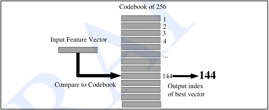
Fig. 2: Overview of VQ

codebook : vocabulary \(V = \{v_{1}, v_{2}, \cdots, v_{n}\}\) 를 구성하는 symbol들의 set, 연속적인 데이터를 이산 데이터로 mapping 되는 집합이며, 이는 기본적으로 vector를 요소로 가지는 리스트이다.
codeword(prototype vector) : codebook 안에 있는 각각의 symbol \(v_{k}\) (e.g., 256개의 codeword를 사용한다면 각각의 vector를 \(0 \sim 255\)로 나타낼 수 있음. 즉, 8-bit 양자화)
clustering algorithm : codebook을 만드는 알고리즘. 학습 set 내의 모든 feature vector들을 256개의 class로 clustering한다. 그러고 나서 이 cluster에서 대표적인 feature vector를 고르고, 이것을 그 cluster에 대한 codeword로 삼는다. 주로 K-means clustering이 자주 사용된다.
distance metric : codebook을 만들고 나면 각각의 input feature vector들을 256개의 codeword와 비교한다. 이때 distance metric을 이용하여 가장 가까운 codeword 하나를 선택한다.