[paper-review] Contrastive Prefence Learning: Learning from Human Feedback without RL
Joey Hejna1, Rafael Rafailov1*, Harshit Sikchi2*, Chelsea Finn1, Scott Niekum3, W. Bradley Knox2, Dorsa Sadigh1 > 1Stanford University, 2UT Austin, 3UMass Amherst * means Equal Contribution
20 Oct 2023
한 문장 요약
요약: Contrastive Leraning objective를 유도하여 Prefernce-based Learning을 수행해보자.
Keyword: Contrastive Learning, Preference-based Learning, Regret
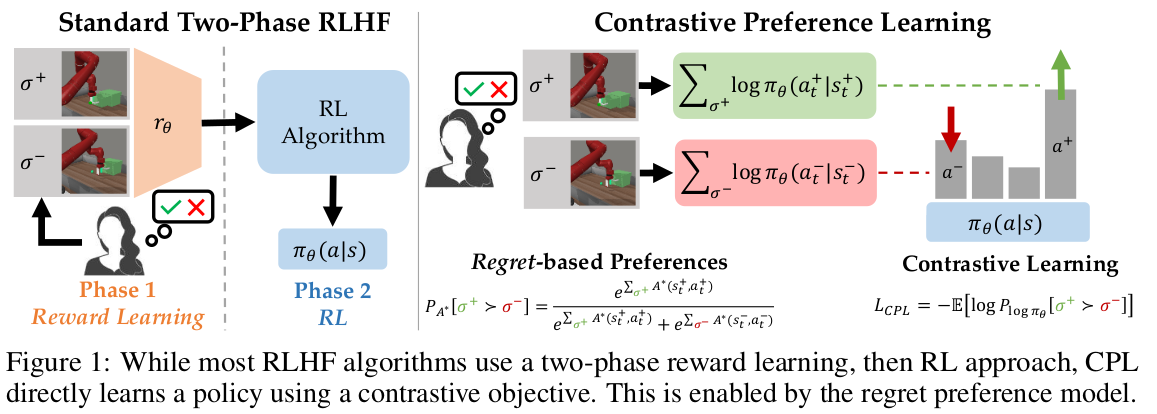
Fig. 1: Overview of the Contrastive Preference Learning (CPL).
Introduction
기존에 수행해오던 Two-Phase RLHF이 가정하고 있는 것에 대해 언급하며 논문이 시작한다.
Human preferences are distributed according to the discounted sum of rewards or partial return of each behavior segment.
최근 연구들은 human으로부터 regret에 기반한 preference feedback을 받는 것으로 새로운 접근을 수행했다.
Positioning that humans instead provide preferences based on the regret of each behavior under the optimal policy of the expert’s reward function.
- Models of human preference for learning reward functions
- Arxiv: https://arxiv.org/abs/2206.02231
- OpenReview: https://openreview.net/forum?id=6UtOXn1LwNE
- NeurIPS rejected ..
즉, Reward 만으로 사람의 optimal choice를 대변해주긴 어렵다고 판단되며, advantage(=negated regret) function으로 feedback에 대해 quantify 하는 것이라고 말함.
그렇게 저자는 Regret-based preference model을 제시하며, 이는 optimal policy에 대한 직접적인 정보를 얻을 수 있는 장점이 있다고 한다. (regret function의 정의에 의해 )
- regret: difference between optimal and actual reward.
저자의 Key insight는 Regret-based Preference framework를 Maximum Entropy와 엮은 것이라고 한다. 그렇게 함으로써 advantage function과 policy를 bijection의 관계로 표현할 수 있다고 한다.
- Bijection: 두 함수 사이를 중복 없이 모두 일대일로 대응하는 함수.
Advantage function 대신 policy 기반으로 최적화 수식을 작성함으로서, 저자는 optimal policy와의 Supervised Learning Objective로 정의할 수 있었다고 한다. 저자는 이를 Contrastive Preference Learning (CPL)이라고 칭하며, 다음 3개의 장점이 있다고 주장합니다.
- CPL can scale as well as supervised learning because it uses only supervised objectives to match the optimal advantage without any policy gradients or dynamic programming.
- CPL is fully off-policy, enabling effectively using any offline sub-optimal data source.
- CPL can be applied to arbitrary Markov Decision Processes (MDPs), allowing for learning from preference queries over sequential data.
Preliminaries
본 논문은 reward-free MDP의 RLHF \(\mathcal{M}/r=(\mathcal{S,A},p,\gamma)\) 를 따른다. 여기서 reward function은 없으니, expert’s preference를 통해 추정해야 한다.
Maximum Entorpy Reinforcement Learning.
Maximum-Entropy RL은 causal entropy를 최대화하는 \(\pi\)를 학습하는 것이 목적이며, 다음의 objective를 가진다.
- \(\alpha\): temperature parameter.
Additional negated \(\log \pi(\cdot)\)는 offline-RL에서 자주 사용되는 항이다. (KL-constrained objective for reference distribution)
The Regret (or Advantage) Preference Model.
Advantage function \(A^{\pi}_{r}(s,a) = Q^{\pi}_{r}(s,a)-V^{\pi}_{r}(s)\) 로 정의되며, policy \(\pi\) 를 따랐을 때 보다 action \(a\) 를 취했을 때에 how worse 한지 파악하는 지표이다. 일반적으로 preference model은 Boltzman rational distribution을 따른다고 하며 연구가 수행되어 왔지만, 이는 partial return을 고려하는 경우에 inconsistent 하다는 연구 결과를 보였다. 혹은 sparse reward에 의해 표현력이 떨어진다는 것도 inconsistent에 영향을 준다고 얘기한다.
Boltzmann rational distribution이란? 어떤 시스템에서 특정 상태 \(i\)에 있을 확률을 해당 상태의 에너지와 시스템의 온도로써 표현하는 것이다. Boltzmann distribution은 아래의 형태를 띈다. \(p*{i} \propto \exp({-\frac{\varepsilon*{i}}{kT}})\)
- \(p_{i}\): state \(i\)에 있을 확률
- \(\epsilon_{i}\): the energy of the state
- \(kT\): Boltzmann constant \(k\), thermodynamic temperature \(T\)
정보이론에 의해 시스템은 낮은 에너지부터 채워지는 경향을 전제로 한다. 즉, 에너지가 낮은 상태의 확률이 에너지가 높은 상태의 확률보다 더 큰 값을 가진다는 의미이다. 쉽게 말해서 energy \(\epsilon_{i}\)의 값이 커질수록 확률값 \(p_{i}\)의 값이 더 낮아진다는 것이다.
Boltzmann distribution은 아래와 같이 정의된다.
\[p*{i} = \frac{1}{Q} \exp({-\frac{\varepsilon*{i}}{kT}}) = \frac{\exp(-\frac{\epsilon*{i}}{kT})}{\sum^{M}*{j=1} \exp(-\frac{\epsilon\_{j}}{kT}{})}\]앞서 작성한 수식과 동일하며, normalization denominator term \(Q\)가 추가된 것이다. \(M\)은 system에서 알 수 있는 모든 state의 수를 의미한다.
reference: wikipedia
기존의 RLHF 방식처럼 partial return을 기준으로 한다면 inconsistency를 띄게 되므로 negated discounted regret segment에 대한 수식으로 표현한다. 그렇게, 이 preference model은 optimal policy를 기준으로 얼마나 lower regret을 보이는지 해석할 수 있다.
\[\begin{equation} P_{A^*}\left[ \sigma^{+} \succ \sigma^{-} \right] = \frac{\exp \sum_{\sigma^{+}} \gamma^{t} A^{\ast}(s^{+}_{t}, a^{+}_{t})}{\exp \sum_{\sigma^{+}}\gamma^{t} A^{\ast}(s^{+}_{t}, a^{+}_{t}) + \exp \sum_{\sigma^{-}}\gamma^{t} A^{\ast}(s^{-}_{t}, a^{-}_{t})} \end{equation}\]- \(+\): preferred behavior segment
- \(-\): unpreferred behavior segment
Contrastive Preference Learning
일반적인 reward model을 사용하는 것은 vast, unnecessary computational expense를 유발한다. 그렇다고 Regret based model이 무조건 다 좋은 것은 아니고, 이 또한 다음의 문제점을 갖고 있다.
- rely on estimating gradients with respect to a moving reward function.
- unsuitable for complex scenarios beyond the simplistic grid world environments.
그렇게 저자는 다음의 Key contribution을 내세운다.
- Max-Ent RL framework에서 Advantage function을 log-probability of the policy로 표현한다.
- Log-probability로 표현하여, 더이상 Advantage function를 학습하지 않아도 된다.
- RL framework에서 수행되던 optimization challenge를 해결하게 된다.
- 즉, aligned regret prefernce를 더욱 근접하게 포착할 수 있고, human feedback을 통해 학습할 때에 supervised learning 만 수행해도 된다는 이점을 갖는다.
- Supervised objective로 변환했다는 것이 핵심적인 contribution 이다.
From Optimal Advantage To Optimal Policy
저자가 제안한 regret preference model은 \(\mathcal{D}_{\text{pref}}\)을 Dataset으로 갖는다.
- \(\mathcal{D}_{\text{pref}}\): Informations about the optimal advantage function \(A^{\ast}(s,a)\)
\(\arg \max\_{a \in \mathcal{A}} A^{\ast}(s,a)=a^{\ast}\) 그러므로 정의에 따라 \(A^{\ast}(\cdot)\) 를 최대화하는 action은 optimal action \(a^{\ast}\) 가 되며 이 \(A^{\ast}(\cdot)\) 함수를 학습한다는 것은 결국 optimal policy \(\pi^{\ast}\)를 반드시 따른다는 것을 알 수 있으며 이는 아래의 수식으로 표현 가능하다.
\[\begin{equation*} \max_{A_{\theta}} \mathbb{E}_{(\sigma^{+},\sigma^{-})\sim \mathcal{D}_{\text{pref}}} \left[ \log P_{A_{\theta}} \left[\sigma^{+} \succ \sigma^{-}\right]\right] \end{equation*}\]쉽게 생각해볼 수 있는 점은, Advantage function을 그대로 Eqn. (2) 에서 parameterized advantage \(A_{\theta}\)로 대체하는 것이다. 하지만 일반적인 RL과 MaxEnt RL 두 경우 모두에 대해서 Bellman-consistent advantage function을 학습하는 것은 non-trivial 하다는 것이다. 즉 학습하기 어려운 경우를 뜻한다.
\(A^{\ast}\)를 \(\pi^{\ast}\)에 대한 관계는 아래와 같다.[Ziebart (2010)] \(\pi^{\ast}\)는 확률 분포의 정의에 따라 \(A^{\ast}\)도 몇 가지 제약 사항을 충족해야만 한다. (probability axioms)
\[\begin{equation*} \pi^{\ast}(a|s) = \exp^{\frac{A^{\ast}_{r}(s,a)}{\alpha}} \end{equation*}\]이는 학습된 \(A^{\ast}\) 가 optimal 하려면, 확률 분포 정의에 의해 normalized 되어야 한다는 것이다. \(\int*{\mathcal{A}} \exp^{\mathcal{A}^{\ast}(s,a)/\alpha}~da = 1\). 이러한 제약 조건은 깊은 신경망과 continuous space 일 경우에 intractable 하게 되므로 \(A*{\theta}\) 를 통해 학습하는 접근(=MLE)은 어려워진다.
그렇다면 \(A_{\theta}\) 를 직접 학습하는 것은 지양해야 한다는 것이며, 다른 방법을 찾아야 한다. 저자는 \(A^{\ast}\) 와 \(\pi^{\ast}\) 의 bijection 성질을 이용해서 수식을 전개해나간다. 이를 통해 \(A^{\ast}\) 이 \(\pi^{\ast}\) 에 log-scale로 비례한다는 의미로 수식을 다시 작성할 수 있다.
\[\begin{equation} A^{\ast}_{r}(s,a) = \alpha \log \pi^{\ast}(a|s) \end{equation}\]이렇게 됨으로써, 우리는 더이상 advantage function을 학습하지 않고, 곧바로 optimal policy를 학습할 수 있게 된다. 즉 Eqn. (3) 을 Eqn. (2)에 대입하면 아래와 같은 수식을 유도할 수 있다.
\[\begin{equation} P_{A^*}[\sigma^{+} \succ \sigma^{-}] = \frac{\exp \sum_{\sigma^{+}} \gamma^{t} \alpha \log \pi^{\ast} (a^{+}_{t} | s^{+}_{t})}{\exp \sum_{\sigma^{+}}\gamma^{t} \alpha \log \pi^{\ast} (a^{+}_{t} | s^{+}_{t}) + \exp \sum_{\sigma^{-}}\gamma^{t} \alpha \log \pi^{\ast} (a^{-}_{t} | s^{-}_{t})} \end{equation}\]이렇게 MaxEnt RL에서 \(\pi^{\ast}\) 만으로 해석할 수 있는 preference model을 유도하게 된다. 위 수식을 토대로 Maximum-Likelihood Estimation(MLE) Loss도 손쉽게 유도할 수 있다.
이렇게 \(\pi_{\theta}\)는 완벽하게 user-preference로 수렴하는 것을 보장하게 된다. 이는 identifiable 이라고 표현된다. (meaning the objective can achieve a loss of zero.)
Assuming sufficient representation power, at convergence \(\pi_{\theta}\) will perfectly model the users preferences, and thus exactly recover \(\pi^{\ast}\) under the advantage-based preference model given an unbounded amount of preference data.
이렇게 supervised manner로 policy를 곧바로 학습하게 되면 다음의 이점을 가질 수 있다.
- circumvents the needs for learning any other functions, like a reward function or value function.
- reduces both complexity and computational cost
- 이전 연구들은 preference model의 shifting distribution 문제점이 있었으나, CPL은 probability axiom에 의해 이러한 문제점을 해결할 수 있다.
- 즉 어떠한 normalization scheme이 필요하지 않다.
- \(\int_{\mathcal{A}} \exp^{\mathcal{A}^{\ast}(s,a)/\alpha}~da = 1\) 성질에 의해 어떠한 reward function에 상응하는 optimal advantage function \(A^{\ast}\)이 존재한다.
- 저자는 이를 consistency 라고 표현하며 Appendix A 에서 증명을 보인다.
Eqn. 2에서 알 수 있듯이 [preferred / unpreferred] 를 \(+\), \(-\)로 표현하고 있으며, 이는 contrastive learning에서 흔히 사용되는 [positive / negative] sample로 이해할 수 있다는 것이다. 저자가 주장하길, Eqn. (5)은 Noise Contrastive Estimation objective로 해석할 수 있으며, Plackett-Luce Model 처럼 Ranking method로 모델링하게 되면 InfoNCE objective 형태로 표현할 수 있다.
</br>
Practical Considerations
이 파트에서는 저자가 실제로 구현할 때에 어떠한 요소들이 학습에 영향을 미쳤는지 분석한 내용을 서술한다.
CPL의 objective가 strictly convex하지 않으며, 이를 logistic regression problem으로 정의하여 해결했다. 우선, policy를 one-dimensional vector로 정의하자. \(\pi \in \mathbb{R}^{\left| \mathcal{S} \times \mathcal{A} \right|}\) 그리고 positive/negative segment를 policy \(\pi\)와 \(\text{comparison}\) vector \(x\)의 \(\text{dot}\) product로 표현할 수 있다.
-
positive segment: $$\sum_{\sigma^{+}} \gamma^{t} \alpha \log \pi_{\theta}(a^{+}_{t} s^{+}_{t})$$ -
negative segment: $$\sum_{\sigma^{-}} \gamma^{t} \alpha \log \pi_{\theta}(a^{-}_{t} s^{-}_{t})$$ - \(\text{comparison}\) vector: \(x_{i}\left[ s,a \right]= \left\{ \begin{matrix} \gamma^{t} & \text{if}~~\sigma^{+}_{i,t}=(s,a) \\ -\gamma^{t} & \text{if}~~\sigma^{-}_{i,t}=(s,a) \\ 0 & \text{otherwise} \\ \end{matrix}\right.\) }
즉 앞서 보았던 Eqn. 5을 logistic function을 사용해서 다시 작성할 수 있다.
- \[\text{logistic}(z)=\frac{1}{1+e^{-z}}\]
Any changes to \(\log \pi\) in the null space of \(X\) have no effect on the logits of the logistic function, and consequently no effect on the loss. In practice, $$\left \mathcal{S \times A}\right » n\(, making the null space of\)X$$ often nontrivial such that there are multiple minimizers of the CPL loss, some of which potentially place a high probability on state-action pairs not in the dataset.
저자는 위에서 언급한 내용을 CPL objective에 regularizer \(\lambda\)를 도입하여 해결한다. 일반적으로 constrastive learning에서 자주 사용되는 휴리스틱이다.
\[\begin{equation} \mathcal{L}_{\text{CPL}\color{red}({\lambda})}(\pi_{\theta}, \mathcal{D}_{\text{pref}}) = \mathbb{E}_{\mathcal{D}_{\text{pref}}}\left[ -\log \frac{\exp \sum_{\sigma^{+}} \gamma^{t} \alpha \log \pi^{\ast} (a^{+}_{t} | s^{+}_{t})}{\exp \sum_{\sigma^{+}} \gamma^{t} \alpha \log \pi^{\ast} (a^{+}_{t} | s^{+}_{t})+\exp {\color{red}({\lambda})}\sum_{\sigma^{-}} \gamma^{t} \alpha \log \pi^{\ast} (a^{-}_{t} | s^{-}_{t})} \right] \end{equation}\]- \[\lambda \in (0,1)\]
negative segment에 대해서 regularizer term을 추가하여 loss가 급격하게 작아지는 것을 방지하고자 한다.
그리고 저자는 behavior cloning 방식으로 \(\pi_{\theta}\)를 pre-train하는 경우가 더 성능이 좋았다고 말한다. 그렇게 저자는 BC로 pre-train 한 후에 CPL로 fine-tuning을 수행하라고 한다.
-
BC objective: $$\min_{\theta} \mathbb{E}{(s,a)\sim \mathcal{D}} \left[ \log \pi{\theta} (a s) \right]$$
Experiments
… 작성 예정.
Thoughts
수식적으로 증명하는 파트가 꽤 있으며, 관련 background에 대해 이해가 높은 상태에서 읽어야 이 논문이 잘 이해될 것 같다. Preference-based Learning을 Contextual Bandit problem으로 수행하는 연구를 진행중이었는데, 이미 이 논문에서 하나의 sub-section에서 다 풀어버린 느낌이다.
기존의 방법들과 달랐던 점은 Advantage function \(A\)를 Regret 개념으로 도입해서, partial return sum에 의존하지 말고, optimal policy와 비교한다는 점이었다. 그리고 \(A\)를 곧바로 학습하는 것이 아니라, policy \(\pi\)로 표현해서 policy를 직접 학습하는 방식이 큰 contribution 이라고 생각한다. (RLHF를 Supervised Learning으로 풀어낸 느낌.)
참 재미있는 연구인 것 같고, 역시 Dorsa 그룹은 대단한 것 같다.
코드를 돌려보려고 했으나, mujoco-py로 개발해두어서 호환성 문제가 생겼다. 얼른 코드를 해석해보자 ..
Enjoy Reading This Article?
Here are some more articles you might like to read next: