[paper-review] Poisson Reconstruction

Eurographics Symposium on Geometry Processing 2006. [Paper]

Michael Kazhdan1¹, Matthew Bolitho¹ and Hugues Hoppe²

¹Johns Hopkins University, Baltimore MD, USA, ²Microsoft Research, Redmond WA, USA

2006

한 문장 요약

요약: Surface reconstruction을 Poisson problem으로 해석해서 수행하자.

0. Reconstruction

이번에 연구 내용으로 수행했던 내용 중 Real-to-Sim 파트가 있었다. 이는 실제 환경의 3D asset의 정보를 미리 정의되어 있는 Asset pool에서 그대로 MuJoCo simulator로 가져오는 그러한 내용이었다. 이 부분을 구현하면서 많은 아쉬움이 있었다. 우선 3D mesh가 이미 정의되어 있어야 한다는 매우 치명적인 한계가 있었다. 그리고 대부분의 Object shape이 cylinder, sphere, flat한 형태였기에 Orientation을 고려할 수 있는 방법이 없었다. 그러던 와중, 최근 각광받느 NeRF 알고리즘 이전에 3D scene reconstruction 연구에선 어떠한 것이 있었는지 공부하고자 글을 작성한다.

1. Introduction

논문은 이와 같은 문장으로 시작한다.

We show that surface reconstruction from oriented points can be cast as a spatial Poisson problem. This Poisson formulation considers all the points at once, without resorting to heuristic spatial partitioning or blending, and is therefore highly resilient to data noise.

우선, 해당 방법론의 입/출력 부터 정의하자면 아래와 같다.

Input : Point cloud with normal (이하 oriented points, sample points, 혹은 그냥 points)
Output : Closed Surface (안과 밖이 명확히 구분 되는 surface. 이하 surface)

우리가 reconstruct 하고자 하는 surface를 다음과 같은 function \(\mathcal{X}\) 으로 생각해볼 수 있다:

\[\begin{equation} \mathcal{X}(x,y,z) \end{equation}\]

점 \((x,y,z)\) 가 surface 내부의 점이면 1, 외부의 점이면 0.

이를 indication function이라 하는데, 이 function \(\mathcal{X}(x,y,z)\) 의 공간 상의 변화율(기울기)인 gradient \(\nabla \mathcal{X}\) 를 구하면, 0에서 1로 바뀌는 순간, 즉 surface 상의 점들에서 0이 아닌 기울기 벡터를 가지게 될 것이다.

기본적으로 이 기울기 vector field는 surface에서 물체 내부로 향하는 normal vector랑 같기 때문에, point cloud with normal은 기울기 벡터 필드로부터 특정 점들에서의 기울기를 sample로 가져온 것이라 볼 수 있다.

즉, 주어진 normal vector를 가진 point set \(\mathrm{V}\)와 가장 유사한 \(\nabla \mathcal{X}\)를 찾아서 \(\nabla \mathcal{X}\) 가 0이 아닌 부분들을 추출한다면 surface를 얻을 수 있다는 접근 방식이다.

\[\begin{equation} \min_{\mathcal{X}} \vert\vert \nabla \mathcal{X} - \vec{V} \vert\vert \end{equation}\]

위 objective를 만족하는 best approximates a vector field \(\vec{V}\) 를 구하기 위해 gradient \(\nabla\) 를 취하면 divergence \(\Delta\) 로 표현되며, 이제 일반적인 Poisson problem으로 치환이 가능하게 된다.

\[\begin{equation} \Delta \mathcal{X} = \nabla \cdot \nabla ~ \mathcal{X} = \nabla \cdot \vec{V} \end{equation}\]

Poisson problem: compute the scalar function \(\mathcal{X}\) whose Laplacian (divergence of gradient) equals the divergence of the vector field. 이렇게 \(V\)로부터 가장 유사한 \(\nabla \mathcal{X}\)를 찾을 때, 다음과 같은 미분 방정식을 세워서 풀게 된다: \(\Delta \mathcal{X} = \nabla \cdot V\) 이 방정식을 푸는 것을 Poisson problem이라 부르며, 이러한 미분 방정식으로 수행하니 Possion Reconstruction이라고 한다.

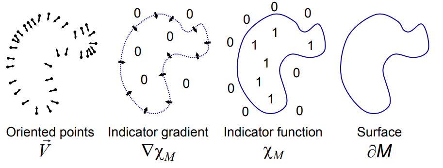
Fig. 1: Intuitive illustration of Poisson reconstruction in 2D.

이렇게 Poisson problem으로 치환하게 되면 아래의 이점을 갖는다고 한다.

기존의 Implicit surface fitting method는 local approx. 이었으며, 부수적인 엔지니어링이 필요했다.

Many implicit surface fitting methods segment the data into regions for local fitting, and further combine these local approximations using blending functions (i.e., RBF approach).
- Poisson reconstruction은 Global solution을 도출하게 되므로, 이러한 고민을 없애주게 되며 그 결과 또한 smooth surface로 표현된다고 한다.
또, 기존 Implicit fitting 방법론들은 오직 sampled point (i.e., oriented points) 부근에서만 수행된다는 단점이 있다.
- Poisson reconstruction은 Global하게 이루어지므로 이 또한 해결된다고 표현한다.

Approach

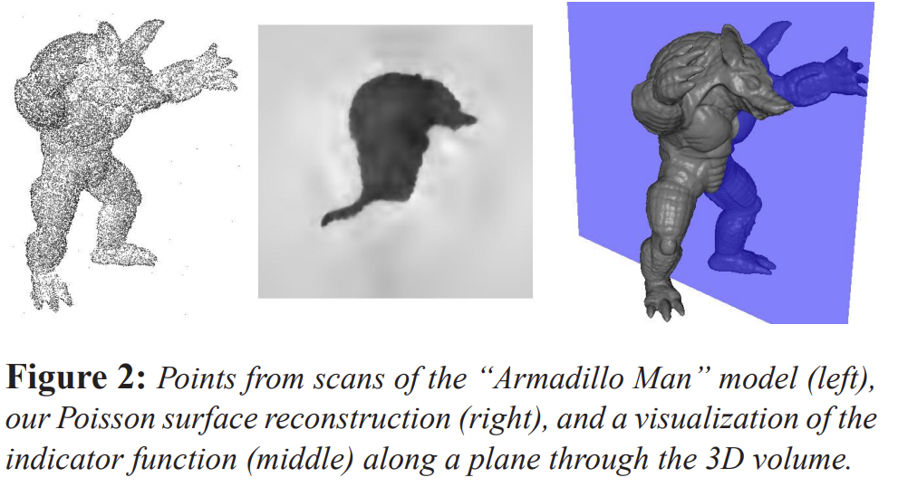
Fig. 2: Overall procedure about Poisson Surface Reconstruction.

\(S\): Input data, set of sampled \(s \in S\)
- each consisting of a point \(s.p\) and an inward-facing normal \(s.\vec{N}\)
\(M\): Unknown surface model, assumed to \(S\) lies on or near the surface \(\partial M\)

Defining the gradient field

목적은 Indicator function을 잘 근사시키는 것이다. 저자는 이를 위해 Gradient Field를 정의하며 시작한다. Indicator function은 \(\{ 0,1 \}\)로 이루어진 piecewise constant function이다. 이에 대한 gradient field를 구하게 되면 표면 부근에 대하여 Unbounded value가 포함되어 있을 것이다. 이를 방지하고자, 저자는 smoothing filter를 고려한 gradient field with a smoothed function Lemma를 제시한다. 이는 smoothed indicator function과 surface normal field에 대한 관계를 표현한 수식이다.

Lemma: Given a solid \(M\) with boundary \(\partial M\), let \(\mathbf{\mathcal{X}_{M}}\) denote the indicator function of \(M\), \(\vec{N}_{\partial M} (p)\) be the inward surface normal at \(p \in \nabla{M},~ \tilde{F}(q)\) be a smoothing filter, and \(\tilde{F}_{p} (q) = \tilde{F}(q-p)\) its translation to the point \(p\). The gradient of the smoothed indicator function is equal to the vector field obtained by smoothing the surface normal field:
\[\begin{equation} \nabla \left( \mathcal{X}_{M} ~ \ast ~ \tilde{F} \right) \left( q_{0} \right) = \int_{\partial M} \tilde{F}_{p} \left( q_{0} \right) \vec{N}_{\partial M} \left( p \right) dp \end{equation}\]

Approximating the gradient field.

입력으로 들어온 oriented point에 대한 integral with discrete summation을 통해 Surface approx.를 수행하게 된다. 구체적으로, 입력 좌표 집합에 대한 여러 patch로 분리하여 (discretize), poisson equation을 세우는 것이다.

\[\begin{equation} \begin{align} \nabla (\mathcal{X}_{M}~\ast~\tilde{F}) (q) &= \sum_{s \in S} \int_{\mathcal{P}_{s}} \tilde{F}_{p} (q) \vec{N}_{\partial M} (p) dP \\ &\approx \sum_{s \in S} \vert \mathcal{P}_{s} \vert \tilde{F}_{s.p} (q) s.\vec{N} \equiv \vec{V}(q) \end{align} \end{equation}\]

\(\mathcal{P}_{S} \subset \partial M\) : Distinct patches
\(\tilde{F}(p)\): smoothing filter

저자가 말하길, Filter를 설정하는 과정에서 고려할 점이 두 가지가 있다고 한다.

It should be sufficiently narrow so that we do not over-smooth the data
It should be wide enough so that the integral over \(\mathcal{P}_{S}\) is well approximated by the value at \(s.p\) scaled by the patch area.

(저자는 위 조건을 만족하는 괜찮은 Filter는 Gaussian으로 사용하는 것을 추천해주었다.)

Solving the Poisson problem

우리가 정의한 Vector field에서 indicator function을 풀어내기 위한 정의가 모두 이루어 졌으며, 이에 대한 exact solution은 일반적으로 항상 존재하지 않는다. (not integrable 하므로, 즉 not curl-free 이다.) 그리하여 아래의 수식에 대해 Least-Square 방식으로 해를 근사시켜 해를 구한다.

\[\begin{equation} \Delta \mathcal{X} = \nabla \cdot \vec{V} \end{equation}\]

Implementation

우리가 구하고자 하는 indicator function은 기본적으로 continuous function(연속 함수)이다. 따라서 특정 point에서의 normal값만을 가진 input Oriented points들을 3d 공간 상의 연속 함수로 변환시키고 난 뒤에, 컴퓨터 상에서 좀더 효율적으로 계산하기 위해 discretize(이산화) 해서 Poisson equation을 세워야한다.

우선은 Input으로 들어온 sample point들을 octree 구조에 배치하고, 각 octree의 node마다 그 안의 점들의 normal vector들의 weighted average를 구하여, 그 node의 normal vector로 삼는다. 이를 Point Rasterization이라고 한다.

이때 Octree는 무조건 정해진 depth의 node로 되어 있는 것이 아니라, sampling density에 따라서 점이 많은 곳은 depth가 높고, 점이 적은 곳은 depth가 낮은 octree를 사용하는 adaptive octree이다. Octree의 node o마다 어떤 function Fo를 associate시켜서, 이 Fo들의 조합으로 전체 vector field V를 표현하고, Poisson equation을 컴퓨터 상에서 풀 수 있는 matrix representation으로 세우고, 최종적으로 풀어서 얻은 indicator function도 이 Fo로 표현되게 한다.

세워진 Poisson equation은 대략적으로 다음과 같은 과정으로 풀이가 된다. 주어진 octree의 depth D에 대해, Poisson solver는 낮은 depth인 0부터 D까지 한단계씩 높이면서, 낮은 depth에서 solution을 찾아 만족시킨 contraint들은 제외시키고 다음 depth에서 조정된 constraint에 맞춰 풀이를 진행한다. 이런 방식을 Cascadic Solver라고 부른다.

현재 쓰이고 있는 Screened Poisson Reconstruction은 Poisson equation을 (∆ - a I)χ = ∇·V 의 형태로 약간 수정한 것인데, 여기서 a값은 기존 Poisson equation의 솔루션 대로 나온 indicator function의 gradient를 중시할 지, 아니면 input으로 넣은 Oriented point들의 배치를 좀더 중시할 지를 따지는 weight값이다. 풀이를 통해 얻은 indicator function의 gradient로부터 marching cubes 알고리즘을 통해 surface를 represent 한다.

Experiments

Poisson Reconstruction 실행시 결과에 영향을 끼치는 다양한 파라미터가 있으나, 가장 결과물에 영향이 큰 것은 다음 세 가지 정도로 볼 수 있다.

Depth / Weight / Sample per Node

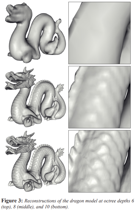
Fig. 3: Varying Octree depth value [6, 8, 10]

Depth가 높을수록 공간을 분할하는 octree의 node의 개수가 많아지므로 더 세밀하게 나눠진 function들로 표현된 indicator function을 얻게 되므로 결과의 해상도가 올라가게 된다. 단, 점의 밀도가 낮을 경우엔 adaptive octree가 그에 맞춰 낮은 depth의 octree를 사용하기 때문에 이것은 사용할 depth의 최대값이라고 보면 된다.

요약

Point cloud를 표현하는 Gradient field를 정의해서 이에 대해 Poisson problem으로 Surface를 표현하는 알고리즘에 대해 공부하였다. 쉽게 비유하자면, Poisson surface reconstruction은은 Implicit mesh representation 방법이며, 이는 매끄러운 천으로 데이터를 감싸는 것으로 설명할 수 있다. Oriented sample 각각이 갖고 있는 Normal의 Surface에 대해서 새로운 point set \(S'\)을 계산하여 기존의 point set \(S\)와 밀접하게 registration 되도록 하는 것이다.

References:

Paper
Code